This post starts from the ordinary derivative and builds to gradient descent for neural networks. If you already know multivariable calculus, you can skip to Why the Gradient is Steepest. If you're here for the ML connection, skip to Applied to Machine Learning. But I'd encourage reading the whole thing — several of the "obvious" steps are where my own misconceptions lived.
Starting from One Dimension
The Derivative as a Rate
You have a function $f(x)$. The derivative $f'(x)$ tells you: if you nudge $x$ by a tiny amount $\Delta x$, how much does $f$ change?
$$f(x + \Delta x) \approx f(x) + f'(x) \cdot \Delta x$$
If $f'(x) > 0$, increasing $x$ increases $f$. If $f'(x) < 0$, increasing $x$ decreases $f$. The magnitude $|f'(x)|$ tells you how sensitive $f$ is to changes in $x$ at that point.
This is the entire foundation. Everything that follows is just asking: what happens when $x$ isn't a single number anymore?
You Can Just Estimate It
Before we even think about formulas, there's a more basic approach. Suppose you have a function $f$ and you don't know its derivative. You can approximate it by just... trying a small step and seeing what happens:
$$f'(x) \approx \frac{f(x + h) - f(x)}{h}$$
Pick a tiny $h$ (say $0.0001$), evaluate $f$ at $x$ and at $x + h$, subtract, divide. That ratio is the slope of a tiny secant line, and as $h$ gets smaller, it converges to the actual derivative. This is the finite difference method, and it's literally how the derivative is defined — the limit as $h \to 0$.
Why mention this? Two reasons. First, it's a sanity check that the derivative isn't some abstract magic — it's the formalization of "nudge the input, measure how much the output changes." Second, it matters for neural networks. In principle, you could compute the gradient of a loss function this way: for each weight, nudge it by $h$, re-run the network, measure how the loss changed. No calculus needed.
The problem is cost. If your network has $n$ parameters, you need $n$ separate forward passes — one per weight. For a model with millions of parameters, that's millions of forward passes per gradient step. Backpropagation (which we'll get to later) computes the exact same gradient in just one forward pass plus one backward pass, regardless of how many parameters there are. That efficiency difference is why backprop exists and why we don't just use finite differences. But finite differences remain useful as a debugging tool — if your backprop implementation is wrong, you can compare its output to the finite-difference estimate to catch bugs.
Finding a Minimum in 1D
If you want to minimize $f(x)$, the derivative tells you which way to step:
$$x_{t+1} = x_t - \eta \cdot f'(x_t)$$
When $f'(x) > 0$, you step left (decreasing $x$). When $f'(x) < 0$, you step right (increasing $x$). The parameter $\eta$ controls how big a step you take. This is gradient descent in one dimension. Simple enough.
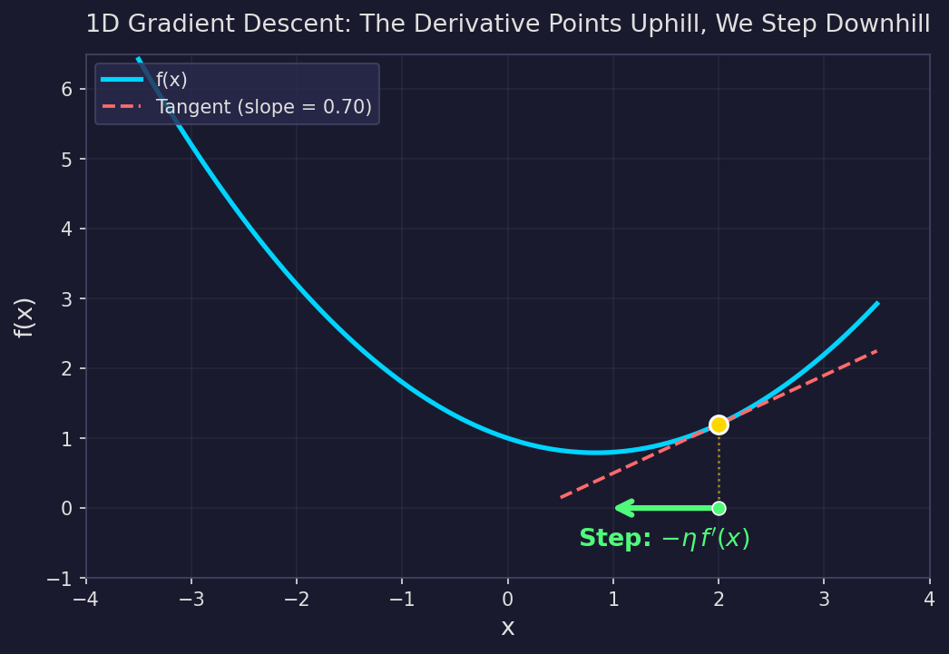
The orange dot is where we currently are. The dashed line is the tangent — its slope is $f'(x)$. The green arrow shows the update direction: opposite to the slope, toward lower values of $f$.
But things get interesting when $f$ depends on more than one input.
Going to Two Dimensions: Partial Derivatives
Now suppose $f(x, y) = x^2 + y^2$. This is a function of two inputs, and its graph is a surface — a bowl sitting in 3D space.
At any point on this surface, we can ask: how does $f$ change if we nudge just $x$, holding $y$ fixed? That gives us the partial derivative $\frac{\partial f}{\partial x} = 2x$. And how does $f$ change if we nudge just $y$, holding $x$ fixed? That gives us $\frac{\partial f}{\partial y} = 2y$.
Geometrically, each partial derivative corresponds to slicing the surface with a plane. $\frac{\partial f}{\partial x}$ is the slope of the curve you get by cutting the surface at constant $y$. $\frac{\partial f}{\partial y}$ is the slope from cutting at constant $x$. Two slices, two slopes.
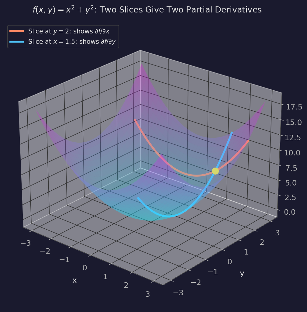
Each colored curve is a parabola — one partial derivative gives the slope of the orange slice, the other gives the slope of the blue slice. At the yellow point, the two slopes together characterize how the surface behaves in every direction. Why? Because any direction in the input plane is just a weighted combination of the $x$ and $y$ directions.
A Misconception I Had to Shake
Here's something that bugged me for a while: why do two partial derivatives tell us everything about the surface at a point? A surface is a 2D object — couldn't there be a whole zoo of different curves running through any given point, each with its own slope, and maybe the surface is some complicated sum of all of them?
The answer is no, and the reason is simple once you see it. The input space is 2D. Any direction you can move in the $xy$-plane can be written as a weighted combination of the $x$-direction and the $y$-direction. There's no third independent direction to go. So any rate of change of $f$ in any direction is determined by the rates of change in the two basis directions — which are exactly the two partial derivatives.
This isn't special to the standard basis either. You could pick any two independent directions, compute the rates of change along those, and recover the rate of change in every other direction. The $x$ and $y$ axes are just convenient.
Directional Derivatives: Any Direction, Not Just the Axes
Partial derivatives tell you the rate of change along the coordinate axes. But you're not limited to stepping along the axes. You can step in any direction.
Pick a unit vector $\mathbf{u} = (u_1, u_2)$ with $u_1^2 + u_2^2 = 1$ — this defines a direction in the input plane. The directional derivative of $f$ in direction $\mathbf{u}$ is:
$$D_{\mathbf{u}} f = \frac{\partial f}{\partial x} u_1 + \frac{\partial f}{\partial y} u_2$$
This says: the rate of change of $f$ in direction $\mathbf{u}$ is a weighted sum of the partial derivatives, with weights given by the components of $\mathbf{u}$.
Parameterizing Direction with an Angle
Since $\mathbf{u}$ is a unit vector in 2D, we can write it as $\mathbf{u} = (\cos\theta, \sin\theta)$ for some angle $\theta$. The directional derivative becomes:
$$D_\theta f = \frac{\partial f}{\partial x} \cos\theta + \frac{\partial f}{\partial y} \sin\theta$$
Now think about what happens as you rotate $\theta$ from $0$ to $2\pi$. At $\theta = 0$ you're looking along the $x$-axis and the directional derivative is just $\frac{\partial f}{\partial x}$. At $\theta = \pi/2$ you're looking along the $y$-axis and it's $\frac{\partial f}{\partial y}$. In between, you get a smooth blend of the two.
The constraint $\cos^2\theta + \sin^2\theta = 1$ is doing important work here. You're not choosing how much to weight each axis independently — the weights are coupled. Putting more weight on $\cos\theta$ (the $x$-component) forces you to put less on $\sin\theta$ (the $y$-component). You're distributing a fixed budget of "step direction" across the axes.
A Concrete Example
Take $f(x,y) = x^2 + y^2$ at the point $(3, 4)$. The partial derivatives are $\frac{\partial f}{\partial x} = 6$ and $\frac{\partial f}{\partial y} = 8$.
The directional derivative as we rotate through $\theta$:
$$D_\theta f = 6\cos\theta + 8\sin\theta$$
At $\theta = 0$ (pure $x$-direction): $D_\theta f = 6$. At $\theta = \pi/2$ (pure $y$-direction): $D_\theta f = 8$. What angle gives the maximum?
If you plot $6\cos\theta + 8\sin\theta$ as a function of $\theta$, you get a sinusoid. It peaks somewhere between $0$ and $\pi/2$ — specifically at $\theta = \arctan(8/6) \approx 53.1°$, where the directional derivative reaches $\sqrt{6^2 + 8^2} = 10$.
That peak direction is exactly the gradient.
The Sinusoid Is Doing More Than You Think
It's worth pausing on why the directional derivative traces out a sinusoid as you rotate. This isn't a coincidence — it's forced by the structure of the problem.
The expression $D_\theta f = f_x \cos\theta + f_y \sin\theta$ is a linear combination of $\cos\theta$ and $\sin\theta$. Any such combination is a pure sinusoid — you can rewrite it as $|\nabla f| \cos(\theta - \theta^)$ where $\theta^$ is the gradient direction. That's just a shifted cosine with amplitude equal to the gradient magnitude. As you spin through all directions at a point, the rate of change sweeps smoothly through one maximum and one minimum per full rotation. No jumps, no flat spots, no complicated multi-peaked landscape. Just a single smooth wave.
This means several things:
There is exactly one steepest-ascent direction and one steepest-descent direction, and they are always $180°$ apart — directly opposite each other. The maximum of the sinusoid is always half a cycle away from the minimum. The gradient and the negative gradient are antipodal. This should feel intuitive (steepest up is opposite steepest down), but the sinusoidal structure makes it airtight: there can't be two unrelated "steep" directions at odd angles to each other, because a sinusoid only has one peak per period.
The transition between them is smooth and monotone over each half-cycle. As you rotate away from the gradient direction, the directional derivative decreases smoothly. There's no direction where it suddenly spikes back up. Every direction between the gradient and the negative gradient has a rate of change strictly between the maximum and minimum.
There is one exception: at a critical point of $f$ — a local minimum, maximum, or saddle point — the gradient is the zero vector. The sinusoid collapses to $D_\theta f = 0$ for all $\theta$. Every direction gives zero rate of change. There is no steepest direction, because the function is (to first order) flat. The maximum and minimum of the directional derivative coincide: both are zero, in every direction. This is the only situation where the "steepest ascent" and "steepest descent" directions are not well-defined.
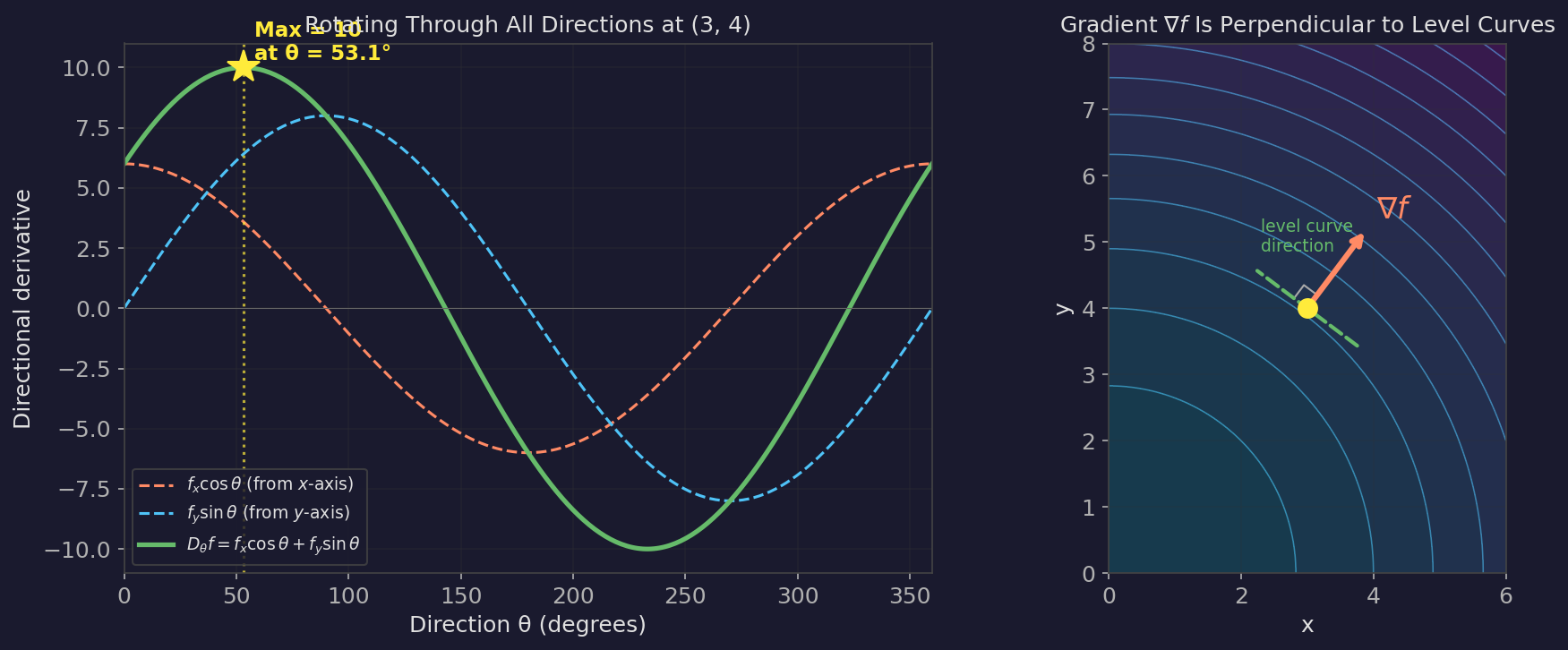
The left panel is the key visual. Watch how $f_x \cos\theta$ (dashed orange) is at its peak at $\theta = 0°$ and falling, while $f_y \sin\theta$ (dashed blue) is rising from zero. Their sum (solid green) peaks at $53.1°$ — not at either axis, but at the optimal tradeoff angle. That angle is where the gradient points. Notice the sinusoid has exactly one peak and one trough per full rotation, $180°$ apart. The right panel shows the same idea geometrically: $\nabla f$ is perpendicular to the level curves, meaning every bit of the step goes toward changing $f$ and none is wasted along the contour.
The Gradient Vector
The gradient of $f$ is the vector of partial derivatives:
$$\nabla f = \left(\frac{\partial f}{\partial x}, \frac{\partial f}{\partial y}\right)$$
In our example at $(3,4)$: $\nabla f = (6, 8)$.
The directional derivative can be written as a dot product:
$$D_{\mathbf{u}} f = \nabla f \cdot \mathbf{u}$$
This compact form is where the key properties come from.
Why the Gradient Is Steepest
This is the central claim: the gradient $\nabla f$ points in the direction of steepest increase. I find it convincing to see this from several angles. I've given four proofs below — the first two build intuition, the last two are more formal. Expand whichever interest you.
Proof 1: Cauchy-Schwarz — the quick formal argument
We want to maximize $D_{\mathbf{u}} f = \nabla f \cdot \mathbf{u}$ over all unit vectors $\mathbf{u}$.
By the Cauchy-Schwarz inequality:
$$\nabla f \cdot \mathbf{u} \leq |\nabla f| \cdot |\mathbf{u}| = |\nabla f|$$
Equality holds when $\mathbf{u}$ is parallel to $\nabla f$. So the maximum directional derivative is $|\nabla f|$, achieved in the direction of $\nabla f$.
Clean and done. But this proof tells you that the gradient is steepest without really telling you why.
Proof 2: The Marginal Gains Argument — the intuitive one (recommended)
Go back to the angle parameterization. We're maximizing:
$$D_\theta f = f_x \cos\theta + f_y \sin\theta$$
where I'm writing $f_x = \frac{\partial f}{\partial x}$ and $f_y = \frac{\partial f}{\partial y}$ to save space.
Think of this as a resource allocation problem. You have a budget of "direction" constrained by $\cos^2\theta + \sin^2\theta = 1$, and you're distributing it between the $x$- and $y$-axes to maximize the total rate of change.
When you're pointing purely in the $x$-direction ($\theta = 0$), your directional derivative is $f_x$. Now start rotating toward $y$ — increasing $\theta$. What happens?
You gain from the $y$-component: $f_y \sin\theta$ is increasing. But you lose from the $x$-component: $f_x \cos\theta$ is decreasing. The gain is worth it as long as the marginal gain from $y$ exceeds the marginal loss from $x$.
The marginal rate of change as you rotate:
$$\frac{d}{d\theta} D_\theta f = -f_x \sin\theta + f_y \cos\theta$$
This is zero when $\tan\theta = \frac{f_y}{f_x}$, which means $\theta = \arctan\left(\frac{f_y}{f_x}\right)$. At that angle, $\mathbf{u}$ is proportional to $(f_x, f_y) = \nabla f$.
The intuition: as you rotate away from one axis toward the other, there are diminishing returns from the axis you're rotating toward (because $\sin\theta$ flattens out near $\pi/2$) and accelerating losses from the axis you're rotating away from (because $\cos\theta$ drops steeply away from $0$). The gradient direction is the exact angle where the marginal gain from rotating further equals the marginal loss. It's the optimal tradeoff point.
Proof 3: The Level Curve Argument — the geometric one
This one is geometric and I find it the most satisfying.
The level curves of $f$ are the curves where $f$ is constant — like contour lines on a topographic map. If you're standing at a point and you move along a level curve, $f$ doesn't change at all. The directional derivative along a level curve is zero.
Now, the gradient is perpendicular to the level curves. (This follows from the fact that $\nabla f \cdot \mathbf{v} = 0$ for any tangent vector $\mathbf{v}$ to the level curve, which is exactly the definition of "the directional derivative along the level curve is zero.")
Why does perpendicularity mean steepest? Because any direction that isn't perpendicular to the level curve has some component along the level curve. That component contributes nothing to changing $f$ — it's wasted movement. The gradient direction is the unique direction that contains no wasted component. Every bit of your step is going toward changing $f$.
Any other direction decomposes into "gradient component" (productive) and "level curve component" (wasted). The gradient itself is the direction with no waste. That's why it's steepest.
Proof 4: Lagrange Multipliers — just optimize it directly
If you prefer computation over geometry, we can maximize $D_\theta f = f_x \cos\theta + f_y \sin\theta$ directly using Lagrange multipliers.
Maximize $g(\mathbf{u}) = f_x u_1 + f_y u_2$ subject to $u_1^2 + u_2^2 = 1$.
$$\mathcal{L} = f_x u_1 + f_y u_2 - \lambda(u_1^2 + u_2^2 - 1)$$
Setting partial derivatives to zero:
$$f_x = 2\lambda u_1, \quad f_y = 2\lambda u_2$$
So $u_1 = \frac{f_x}{2\lambda}$ and $u_2 = \frac{f_y}{2\lambda}$. Plugging into the constraint gives $\lambda = \frac{1}{2}|\nabla f|$, and the optimal direction is $\mathbf{u} = \frac{\nabla f}{|\nabla f|}$. The gradient direction, again.
Wait — Steepest Under What Norm?
Here's something that bugged me once I noticed it, and I think it's one of the most underappreciated points in all of optimization.
Every proof above has the constraint $u_1^2 + u_2^2 = 1$. That's the Euclidean (L2) norm — the ordinary straight-line distance. The set of all unit vectors under this norm is a circle. The gradient is the steepest direction on that circle.
But step back and ask: why a circle? What makes "Euclidean distance" the right way to measure step size?
Nothing, actually. It's a choice. And if you choose differently, the answer to "which direction is steepest?" changes completely.
Let's try the L1 (Manhattan) norm instead. Under L1, a "unit step" means $|u_1| + |u_2| = 1$. Think about what that looks like: instead of a circle, the set of unit vectors is a diamond — a square rotated $45°$, with its corners sitting on the coordinate axes at $(\pm 1, 0)$ and $(0, \pm 1)$.
Now we want to maximize the same linear objective: $D_\mathbf{u} f = f_x u_1 + f_y u_2$, but subject to the L1 constraint.
Let's think about why this forces the answer to a coordinate axis. Take any point on the L1 diamond that isn't a corner — say $(0.5, 0.5)$, which satisfies $|0.5| + |0.5| = 1$. The objective value there is $6(0.5) + 8(0.5) = 7$. But we could redistribute that budget: move weight from $u_1$ toward $u_2$. Try $(0.3, 0.7)$: objective is $6(0.3) + 8(0.7) = 7.4$. Better. Keep going — $(0.1, 0.9)$: objective is $6(0.1) + 8(0.9) = 7.8$. Still improving. All the way to the corner at $(0, 1)$: objective is $6(0) + 8(1) = 8$.
Every time we shift weight from the weaker axis ($f_x = 6$) to the stronger axis ($f_y = 8$), we gain more than we lose. This will always be true: as long as one partial derivative is strictly larger than the other, the optimal move is to go all-in on the bigger one. On the L1 diamond, you can go all-in — that's what the corners are. On the L2 circle, you can't — the curvature of the circle forces blending.
This is a general fact: a linear function maximized over a convex polytope (a shape with flat faces and sharp corners) always achieves its max at a vertex. The L1 ball is a polytope; the L2 ball isn't. That geometric difference is the entire reason the two norms give different answers.
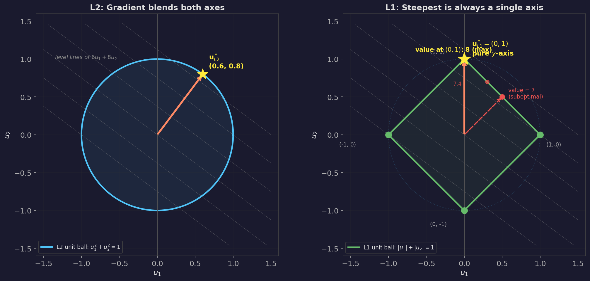
The L1 corners are just the pure axis directions: $(1, 0)$, $(-1, 0)$, $(0, 1)$, $(0, -1)$. So:
Under L1, "steepest ascent" means: find the single coordinate with the largest absolute partial derivative, and step entirely along that axis. Ignore all other coordinates.
$$\mathbf{u}{L1}^* = \text{sign}!\left(f{k}\right) \cdot \mathbf{e}_k \quad \text{where } k = \arg\max_j |f_j|$$
No blending. No smooth tradeoff. Just: which axis matters most? Go that way. Everything else gets zero.
In our running example at $(3, 4)$ with $f_x = 6$ and $f_y = 8$:
- L2 answer: Blend both axes. Step in the direction $(6, 8)/10 = (0.6, 0.8)$, at $53.1°$ between the axes.
- L1 answer: Step purely along $y$. Direction $(0, 1)$. Ignore $x$ entirely, because $|f_y| > |f_x|$.
Same function, same point, same partial derivatives — completely different "steepest" directions. The difference isn't in the function. It's in what you mean by "one step."
Why This Matters Beyond Math
This isn't a curiosity. It connects several things that are usually taught as unrelated:
Coordinate descent — the optimization algorithm where you update one parameter at a time, cycling through them — is L1-steepest descent. When you ask "which single parameter should I change to improve the objective most?", you're doing exactly the L1 optimization above. It's a perfectly valid optimization strategy, and it's the natural strategy if your cost budget is "one parameter change" rather than "one Euclidean step."
L1 regularization (Lasso) promotes sparse solutions — solutions where many parameters are exactly zero. Now you can see why: the L1 ball has sharp corners on the axes. When you constrain or penalize the L1 norm of your parameter vector, the optimizer tends to land at those corners, which correspond to parameters being exactly zero. The same geometric fact that makes L1-steepest descent axis-aligned (go all-in on one axis, ignore the rest) also makes L1-regularized solutions sparse (keep a few parameters, zero out the rest). The sparsity isn't a trick. It's the geometry.
The gradient is only "steepest" relative to a norm. When a textbook says "the gradient is the direction of steepest ascent," there's a silent "under the Euclidean norm" attached. Standard gradient descent is L2 optimization. This isn't wrong — L2 is the default for good reasons (rotationally invariant, differentiable, natural for inner-product spaces). But it's a convention, not a theorem about the universe. Knowing that it's a choice opens the door to understanding why different optimizers exist and when they're appropriate.
Misconceptions Worth Clearing Up
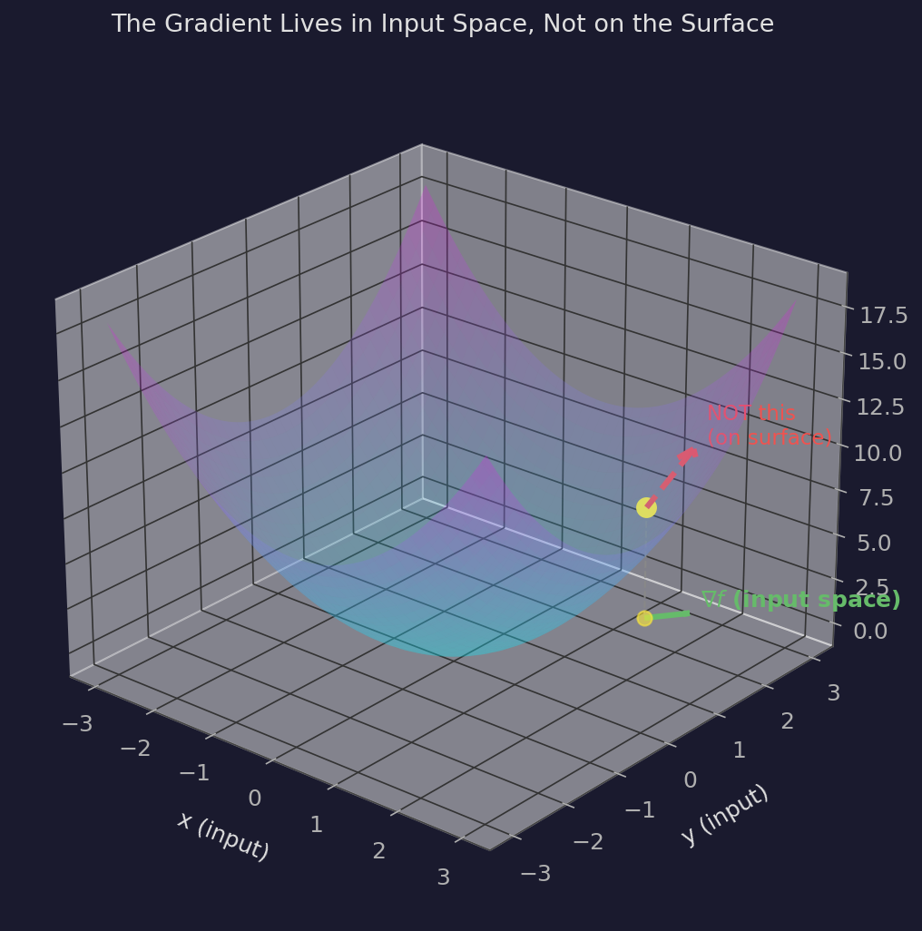
The Gradient Does Not Point "Uphill on the Surface"
This was my biggest wrong mental model for longer than I'd like to admit.
When you visualize a surface $z = f(x,y)$ in 3D, it's natural to imagine the gradient as an arrow pointing "uphill" on that surface — like a ball rolling uphill. But that's not what the gradient is. The gradient lives in the input space, not on the surface.
The gradient $\nabla f = (f_x, f_y)$ is a 2D vector in the $xy$-plane. It points in the input direction that causes $f$ to increase fastest. It has nothing to say about the $z$-direction. The "slope of the surface" is a 3D concept; the gradient is a 2D object.
This matters because when you do gradient descent, you're updating inputs (parameters), not moving along the surface. You're in parameter space, picking a direction to step. The gradient tells you which input direction produces the steepest change in the output. It doesn't "live on" the loss landscape — it lives in the space you're navigating.
The Gradient Is Local — It Tells You Nothing About the Step You're About to Take
The gradient $\nabla f$ at a point $\mathbf{x}$ is a linear approximation. It says: if you were to take an infinitesimally small step in direction $\mathbf{u}$, the rate of change would be $\nabla f \cdot \mathbf{u}$.
It says nothing about what happens when you take a step of actual finite size. The surface could curve, twist, or drop off a cliff one step away and the gradient at your current point wouldn't know. It's a local tangent, not a trajectory.
This is why learning rate matters so much. The gradient points in a direction that's correct locally — but if your step size is too large, you overshoot the region where that linear approximation holds and end up somewhere the gradient wasn't telling you about.
Think of it this way: the gradient is a compass bearing taken from where you're standing. It tells you which direction is downhill right here. It doesn't tell you whether there's a ravine fifty meters ahead that the bearing would walk you straight into.
The Negative Gradient Is Steepest Descent
If $\nabla f$ is the direction of steepest increase, then $-\nabla f$ is the direction of steepest decrease. This is just flipping the sign: the directional derivative $\nabla f \cdot \mathbf{u}$ is most negative when $\mathbf{u}$ points opposite to $\nabla f$.
Gradient descent follows $-\nabla f$. This should feel obvious, but it's worth saying explicitly because the sign convention trips people up when they start reading papers.
Applied to Machine Learning
Here's where all of this connects to training neural networks.
The Network as a Function of Two Things
A neural network is a function. It takes an input $\mathbf{x}$ (your data) and produces a prediction $\hat{y}$. But that function is also shaped by parameters $\theta$ (the weights and biases). So the full picture is:
$$\hat{y} = f(\mathbf{x};; \theta)$$
Read this as: "the prediction $\hat{y}$ is a function of the input $\mathbf{x}$, parameterized by $\theta$." The semicolon is doing real work — it separates the things you feed in (data) from the things you tune (weights).
The loss function then measures how far off that prediction is from the true target $y^*$:
$$\mathcal{L} = L!\left(f(\mathbf{x};; \theta),; y^*\right)$$
or writing it compactly:
$$\mathcal{L}(\theta;; \mathbf{x}, y^*)$$
This is a function of both the parameters and the data. This is a point I want to stress because it's easy to lose track of. The loss has two kinds of arguments, and they play very different roles.
What Can You Change?
You can't change the training data — it's given to you. You can change the parameters $\theta$. So when you compute the gradient, you compute it with respect to $\theta$ only, treating the data as fixed:
$$\nabla_\theta \mathcal{L} = \nabla_\theta , L!\left(f(\mathbf{x};; \theta),; y^*\right)$$
This asks: holding this data point fixed, in which direction should I nudge the weights to reduce the loss the most?
The loss surface you're descending has one dimension for every parameter in the network. For a model with 10 million parameters, you're navigating a 10-million-dimensional surface. The gradient at your current weights is a 10-million-dimensional vector pointing in the direction of steepest increase on that surface. You step in the negative gradient direction.
The Loss Surface Depends on the Data
Here's the thing that took me a while to internalize. The loss surface isn't a fixed landscape you're exploring. It's a landscape that depends on which data points you're evaluating on.
If you lock in one training example $(\mathbf{x}_1, y_1^)$, you get one loss surface. If you lock in a different example $(\mathbf{x}_2, y_2^)$, you get a different loss surface — same parameters, different terrain. The gradient on the first surface might point in a completely different direction than the gradient on the second.
Single Point, Batch, and Stochastic
For a single training example, the loss and gradient are:
$$\mathcal{L}(\theta;; \mathbf{x}i, y_i^) = L!\left(f(\mathbf{x}_i;; \theta),; y_i^\right), \qquad \nabla\theta \mathcal{L}(\theta;; \mathbf{x}_i, y_i^*)$$
In full-batch gradient descent, you average over the entire training set of $N$ examples:
$$\mathcal{L}{\text{batch}}(\theta) = \frac{1}{N}\sum{i=1}^{N} L!\left(f(\mathbf{x}_i;; \theta),; y_i^*\right)$$
The gradient of the average is the average of the gradients:
$$\nabla_\theta \mathcal{L}{\text{batch}} = \frac{1}{N}\sum{i=1}^{N} \nabla_\theta , L!\left(f(\mathbf{x}_i;; \theta),; y_i^*\right)$$
This gives you the "true" gradient — the direction that reduces the loss on average across all training data. In practice, this is expensive when $N$ is large. So we use mini-batches: sample a subset $\mathcal{B} \subset {1, \ldots, N}$ and approximate:
$$\nabla_\theta \mathcal{L}{\text{batch}} \approx \frac{1}{|\mathcal{B}|}\sum{i \in \mathcal{B}} \nabla_\theta , L!\left(f(\mathbf{x}_i;; \theta),; y_i^*\right)$$
This is stochastic gradient descent (SGD). Different mini-batch, different estimate, different step direction. The extreme case is a batch size of 1: pick one training point, compute its gradient, step. That's pure stochastic gradient descent, and it's what we'll work through by hand in the next section.
Why This Approximation Works
There's a natural question here: if we're only using a fraction of the data each step, why should the mini-batch gradient be anywhere close to the true full-batch gradient?
The answer comes from basic statistics. If you pick training examples randomly (uniformly, without bias), then the gradient computed on your mini-batch is an unbiased estimator of the true gradient. In plain language: on any single mini-batch, your gradient estimate might be off — it might point somewhat left of the true direction, or somewhat right. But on average, across many random mini-batches, the errors cancel out. The expected value of the mini-batch gradient equals the full-batch gradient.
This is the same principle behind polling. If you want to know the average height of everyone in a city, you don't need to measure every person. Pick a random sample, compute the average, and the law of large numbers guarantees that your sample average converges to the true average as the sample grows. The larger your mini-batch, the more precise your estimate — but even a small mini-batch points in roughly the right direction, in expectation.
The key requirement is random sampling. If you chose your mini-batches non-randomly — say, always training on the easiest examples first — the estimator would be biased, and the gradient would systematically point in the wrong direction. This is why shuffling the training data each epoch matters: it ensures that each mini-batch is a representative random sample of the full dataset, so the mini-batch gradient is an honest (unbiased) estimate of the full-batch gradient.
The Noise Is Actually Helpful
You'd think noisy gradients would be strictly worse than exact gradients. But empirically, the noise from mini-batch sampling helps. It acts as a form of regularization — the random perturbation makes it harder for the optimizer to settle into sharp, narrow minima that overfit the training data. Instead, the noise pushes you toward broader, flatter minima that tend to generalize better.
This is one of those cases where the theoretically "correct" approach (full-batch exact gradients) is worse in practice than the noisy approximation. The imperfection is load-bearing.
What "Goodness" Means Depends on the Loss Function
The gradient points in the direction of steepest decrease of $\mathcal{L}$. But what counts as "good" — what it means for the loss to be small — is entirely determined by your choice of loss function. Mean squared error, cross-entropy, contrastive losses — these define different surfaces, different gradients, different notions of improvement. The gradient doesn't know what you're trying to achieve. It just knows which way is downhill on whatever surface you gave it. Choosing the right loss function is choosing the right definition of "better."
We Assume a Minimum Exists
All of this implicitly assumes that following the negative gradient actually leads somewhere useful — that there's a minimum to find. This isn't guaranteed by the math alone. It's guaranteed (or at least made plausible) by the choice of loss function. We pick loss functions that are bounded below (the loss can't go negative) and that have well-behaved geometry. If you chose a loss function with no minimum, gradient descent would wander forever.
In practice, modern loss functions for neural networks behave well enough. The surface has minima. Gradient descent finds them. The interesting questions are about which minimum you end up in and whether it generalizes — but the basic existence of something to converge toward is usually not in doubt.
Worked Example: One SGD Step on a Tiny Network
Let's make all of this concrete. We'll build a small network, pick one training point, and compute everything by hand — forward pass, loss, every single gradient, and the weight update.
The Network
Architecture: 1 input → 3 hidden neurons (ReLU) → 1 output (linear). No biases, to keep the arithmetic clean.
| |
The six parameters are:
| Parameter | Layer | Connects | Initial Value |
|---|---|---|---|
| $w_1^{(1)}$ | 1 | input → $h_1$ | $0.5$ |
| $w_2^{(1)}$ | 1 | input → $h_2$ | $-0.3$ |
| $w_3^{(1)}$ | 1 | input → $h_3$ | $0.8$ |
| $w_1^{(2)}$ | 2 | $h_1$ → output | $0.4$ |
| $w_2^{(2)}$ | 2 | $h_2$ → output | $-0.6$ |
| $w_3^{(2)}$ | 2 | $h_3$ → output | $0.2$ |
Training point (batch size = 1): $;x = 2.0, \quad y^* = 1.0$
Loss function: MSE $= (\hat{y} - y^*)^2$
Learning rate: $\eta = 0.1$
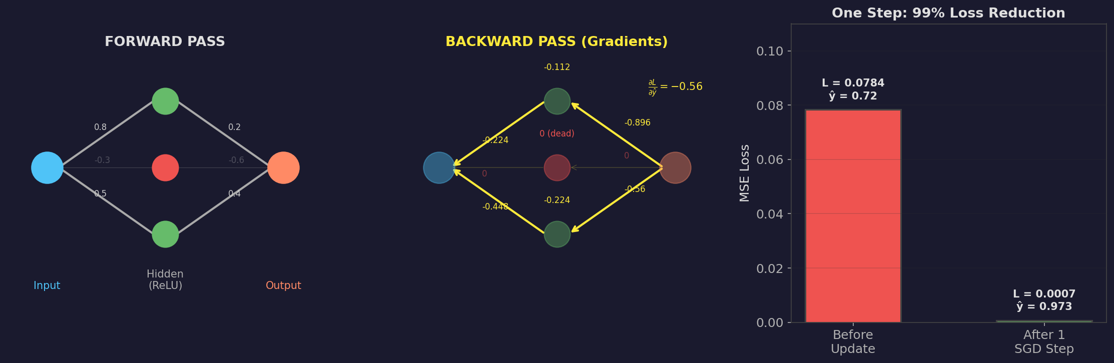
Forward Pass
Layer 1 — compute pre-activations (linear):
$$z_1 = w_1^{(1)} \cdot x = 0.5 \times 2.0 = 1.0$$ $$z_2 = w_2^{(1)} \cdot x = -0.3 \times 2.0 = -0.6$$ $$z_3 = w_3^{(1)} \cdot x = 0.8 \times 2.0 = 1.6$$
Apply ReLU: $;\text{ReLU}(z) = \max(0, z)$
$$h_1 = \text{ReLU}(1.0) = 1.0$$ $$h_2 = \text{ReLU}(-0.6) = 0 \quad \leftarrow \text{killed}$$ $$h_3 = \text{ReLU}(1.6) = 1.6$$
Neuron 2 is dead for this input. Its ReLU output is zero, so it contributes nothing to the output and (as we'll see) receives no gradient. This is a real phenomenon — "dead neurons" in ReLU networks.
Layer 2 — compute output (linear, no activation):
$$\hat{y} = w_1^{(2)} h_1 + w_2^{(2)} h_2 + w_3^{(2)} h_3 = 0.4 \times 1.0 + (-0.6) \times 0 + 0.2 \times 1.6 = 0.72$$
Loss:
$$\mathcal{L} = (\hat{y} - y^*)^2 = (0.72 - 1.0)^2 = (-0.28)^2 = 0.0784$$
We predicted $0.72$, the target is $1.0$. Now: which direction should we nudge each of the six weights to fix this?
Backward Pass (Backprop)
We work backwards from the loss, applying the chain rule at each step.
Step 1: Gradient of loss with respect to the output.
$$\frac{\partial \mathcal{L}}{\partial \hat{y}} = 2(\hat{y} - y^*) = 2(0.72 - 1.0) = -0.56$$
The negative sign tells us: increasing $\hat{y}$ would decrease the loss. Makes sense — our prediction is too low.
Step 2: Gradients for the output layer weights. Since $\hat{y} = \sum_j w_j^{(2)} h_j$:
$$\frac{\partial \mathcal{L}}{\partial w_j^{(2)}} = \frac{\partial \mathcal{L}}{\partial \hat{y}} \cdot h_j$$
| Weight | Gradient | Calculation |
|---|---|---|
| $w_1^{(2)}$ | $-0.56 \times 1.0 = -0.56$ | $h_1$ was active, strong gradient |
| $w_2^{(2)}$ | $-0.56 \times 0 = 0$ | $h_2$ was dead, zero gradient |
| $w_3^{(2)}$ | $-0.56 \times 1.6 = -0.896$ | $h_3$ was active and large, biggest gradient |
Notice: $w_2^{(2)}$ gets zero gradient because its input $h_2$ was zero. The weight can't help reduce the loss if the neuron feeding it is dead.
Step 3: Backpropagate through the hidden layer. First, how much does the loss care about each hidden neuron's output?
$$\frac{\partial \mathcal{L}}{\partial h_j} = \frac{\partial \mathcal{L}}{\partial \hat{y}} \cdot w_j^{(2)}$$
| Neuron | $\frac{\partial \mathcal{L}}{\partial h_j}$ | Calculation |
|---|---|---|
| $h_1$ | $-0.56 \times 0.4 = -0.224$ | |
| $h_2$ | $-0.56 \times (-0.6) = 0.336$ | |
| $h_3$ | $-0.56 \times 0.2 = -0.112$ |
Step 4: Backpropagate through ReLU. The derivative of ReLU is 1 if the input was positive, 0 otherwise:
$$\frac{\partial \mathcal{L}}{\partial z_j} = \frac{\partial \mathcal{L}}{\partial h_j} \cdot \text{ReLU}'(z_j) = \begin{cases} \frac{\partial \mathcal{L}}{\partial h_j} & \text{if } z_j > 0 \\ 0 & \text{if } z_j \leq 0 \end{cases}$$
| Neuron | $z_j$ | ReLU' | $\frac{\partial \mathcal{L}}{\partial z_j}$ |
|---|---|---|---|
| 1 | $1.0 > 0$ | $1$ | $-0.224$ |
| 2 | $-0.6 \leq 0$ | $0$ | $0$ ← gradient killed |
| 3 | $1.6 > 0$ | $1$ | $-0.112$ |
This is the ReLU gradient gate in action. Neuron 2 was inactive during the forward pass, so during the backward pass it blocks the gradient entirely. No learning signal reaches $w_2^{(1)}$ through this path.
Step 5: Gradients for the input layer weights. Since $z_j = w_j^{(1)} \cdot x$:
$$\frac{\partial \mathcal{L}}{\partial w_j^{(1)}} = \frac{\partial \mathcal{L}}{\partial z_j} \cdot x$$
| Weight | Gradient | Calculation |
|---|---|---|
| $w_1^{(1)}$ | $-0.224 \times 2.0 = -0.448$ | |
| $w_2^{(1)}$ | $0 \times 2.0 = 0$ | dead neuron, no update |
| $w_3^{(1)}$ | $-0.112 \times 2.0 = -0.224$ |
The Full Gradient
Collecting everything, the gradient of the loss with respect to all six weights is:
$$\nabla_\theta \mathcal{L} = \begin{pmatrix} \partial \mathcal{L}/\partial w_1^{(1)} \\ \partial \mathcal{L}/\partial w_2^{(1)} \\ \partial \mathcal{L}/\partial w_3^{(1)} \\ \partial \mathcal{L}/\partial w_1^{(2)} \\ \partial \mathcal{L}/\partial w_2^{(2)} \\ \partial \mathcal{L}/\partial w_3^{(2)} \end{pmatrix} = \begin{pmatrix} -0.448 \\ 0 \\ -0.224 \\ -0.56 \\ 0 \\ -0.896 \end{pmatrix}$$
This is a single vector in 6-dimensional parameter space. It's the direction of steepest increase of the loss. We step in the opposite direction.
The Update
$$\theta_{t+1} = \theta_t - \eta , \nabla_\theta \mathcal{L}$$
| Weight | Before | $-\eta \times$ Gradient | After |
|---|---|---|---|
| $w_1^{(1)}$ | $0.5$ | $-0.1 \times (-0.448) = +0.0448$ | $0.5448$ |
| $w_2^{(1)}$ | $-0.3$ | $-0.1 \times 0 = 0$ | $-0.3$ |
| $w_3^{(1)}$ | $0.8$ | $-0.1 \times (-0.224) = +0.0224$ | $0.8224$ |
| $w_1^{(2)}$ | $0.4$ | $-0.1 \times (-0.56) = +0.056$ | $0.456$ |
| $w_2^{(2)}$ | $-0.6$ | $-0.1 \times 0 = 0$ | $-0.6$ |
| $w_3^{(2)}$ | $0.2$ | $-0.1 \times (-0.896) = +0.0896$ | $0.2896$ |
All the negative gradients produced positive updates — the weights moved in the direction that increases $\hat{y}$, which is correct since our prediction was too low. The two weights connected to the dead neuron ($w_2^{(1)}$ and $w_2^{(2)}$) didn't change at all.
Did It Work?
Run the forward pass again with the updated weights:
$$z_1 = 0.5448 \times 2.0 = 1.090, \quad z_3 = 0.8224 \times 2.0 = 1.645$$ $$h_1 = 1.090, \quad h_2 = 0, \quad h_3 = 1.645$$ $$\hat{y}_{\text{new}} = 0.456 \times 1.090 + 0 + 0.2896 \times 1.645 = 0.497 + 0.476 = 0.973$$
$$\mathcal{L}_{\text{new}} = (0.973 - 1.0)^2 = 0.00073$$
One step took the loss from $0.0784$ to $0.00073$ — a 99% reduction. The prediction moved from $0.72$ to $0.973$, nearly hitting the target of $1.0$.
We can visualize this on the loss surface. Our network has 6 weights, so the full loss surface is 6-dimensional — impossible to plot. But we can take a 2D slice by fixing four weights at their initial values and varying only $w_1^{(2)}$ and $w_3^{(2)}$ (the two active output-layer weights):
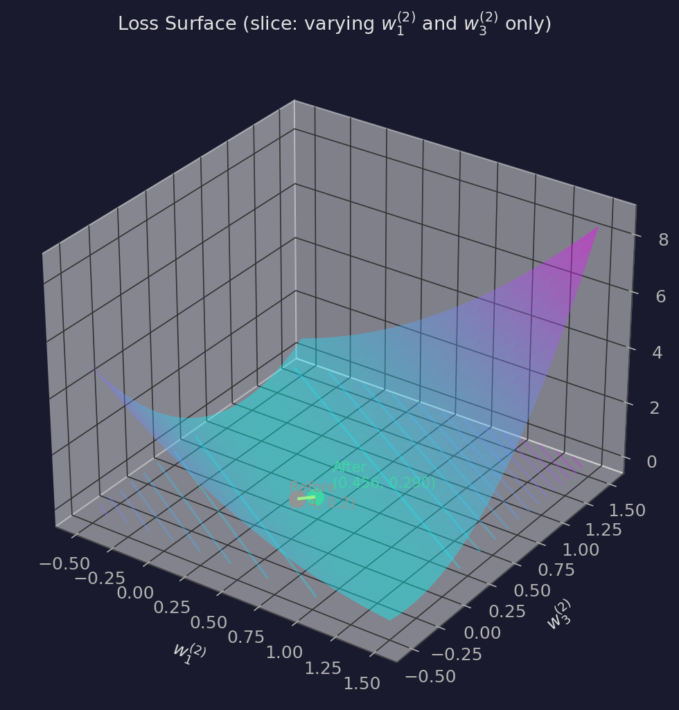
The valley floor is the set of $(w_1^{(2)}, w_3^{(2)})$ pairs where $w_1^{(2)} \cdot 1.0 + w_3^{(2)} \cdot 1.6 = 1.0$ — all the weight combinations that perfectly predict the target. The gradient step moved us almost directly toward this valley.
This is a single stochastic gradient step on a single data point. It worked dramatically well here because we have very few parameters and one data point — the network can almost perfectly fit it in one step. In practice, with millions of parameters and thousands of data points pulling in different directions, progress per step is much smaller and much noisier. But the mechanism is exactly the same: compute the gradient, step opposite to it, repeat.
The Update Rule
Putting it all together, one step of gradient descent for training a neural network:
- Forward pass: Given current parameters $\theta_t$ and a batch of training data, compute the network's predictions and the loss $\mathcal{L}(\theta_t)$.
- Backward pass (backprop): Compute $\nabla_\theta \mathcal{L}$ — the gradient of the loss with respect to every parameter.
- Update: $\theta_{t+1} = \theta_t - \eta \nabla_\theta \mathcal{L}(\theta_t)$
Repeat until the loss is small enough or you run out of patience.
What Backpropagation Actually Is
Backprop is often conflated with gradient descent, and they're not the same thing. Gradient descent is the optimization algorithm — it says "step opposite the gradient." Backpropagation is the algorithm that computes the gradient efficiently. You could compute the gradient other ways (and people did, before backprop became standard). Backprop just happens to be dramatically faster.
A neural network is a composition of functions: layer after layer of linear transformations and nonlinearities. The loss is a function of the output, which is a function of the last layer's output, which is a function of the previous layer, and so on. To get $\nabla_\theta \mathcal{L}$, you need the chain rule.
For a network $f = f_n \circ f_{n-1} \circ \ldots \circ f_1$:
$$\frac{\partial \mathcal{L}}{\partial \theta_i} = \frac{\partial \mathcal{L}}{\partial f_n} \cdot \frac{\partial f_n}{\partial f_{n-1}} \cdots \frac{\partial f_{i+1}}{\partial f_i} \cdot \frac{\partial f_i}{\partial \theta_i}$$
If you look at this formula for different parameters $\theta_i$, you'll notice something: the expressions share a lot of structure. $\frac{\partial \mathcal{L}}{\partial \theta_n}$ needs just one multiplication. $\frac{\partial \mathcal{L}}{\partial \theta_{n-1}}$ needs the same factor $\frac{\partial \mathcal{L}}{\partial f_n}$ plus one more multiplication. And $\frac{\partial \mathcal{L}}{\partial \theta_1}$ needs the entire chain.
Backpropagation exploits this by computing from right to left — starting at the loss and working backward — so that each intermediate derivative $\frac{\partial \mathcal{L}}{\partial f_k}$ is computed once and reused for every parameter in layers $k$ and earlier. That reuse is what makes it efficient.
Why Not Just Estimate the Gradient?
Earlier we saw that you can approximate a derivative with finite differences: bump a parameter by a tiny $\varepsilon$, re-run the network, see how the loss changes. For a single parameter:
$$\frac{\partial \mathcal{L}}{\partial \theta_i} \approx \frac{\mathcal{L}(\theta_i + \varepsilon) - \mathcal{L}(\theta_i)}{\varepsilon}$$
This works. But to get the gradient of all $P$ parameters, you need to do this $P$ times — one forward pass per parameter. Each forward pass walks through all $n$ layers.
Cost of finite differences: $P$ forward passes $\times$ $n$ operations each $= O(P \cdot n)$.
Now consider backprop: one forward pass ($n$ operations) plus one backward pass ($n$ operations).
Cost of backprop: $O(n)$ — independent of the number of parameters.
For a modern language model with billions of parameters, this is the difference between "feasible" and "physically impossible." Finite differences on GPT-3's 175 billion parameters would require 175 billion forward passes per training step. Backprop needs two.
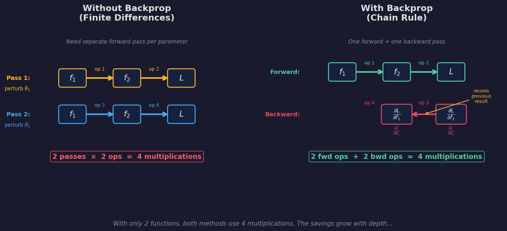
Seeing the Savings: A Chain of 2
Let's make this concrete with a tiny example. Consider a chain of just two functions, each with one parameter:
$$x \xrightarrow{f_1(\theta_1)} a \xrightarrow{f_2(\theta_2)} \hat{y} \xrightarrow{\mathcal{L}} \text{loss}$$
Without backprop — to get both partial derivatives by finite differences, you need:
- Perturb $\theta_1$, run $f_1 \to f_2 \to \mathcal{L}$: 2 operations
- Perturb $\theta_2$, run $f_1 \to f_2 \to \mathcal{L}$: 2 operations
- Total: 4 operations (2 passes × 2 ops)
With backprop:
- Forward: $f_1 \to f_2 \to \mathcal{L}$: 2 operations
- Backward: compute $\frac{\partial \mathcal{L}}{\partial \hat{y}}$, then $\frac{\partial \mathcal{L}}{\partial a} = \frac{\partial \mathcal{L}}{\partial \hat{y}} \cdot \frac{\partial f_2}{\partial a}$: 2 operations
- Total: 4 operations (1 forward + 1 backward)
With only 2 parameters, the cost is the same. The savings come from depth.
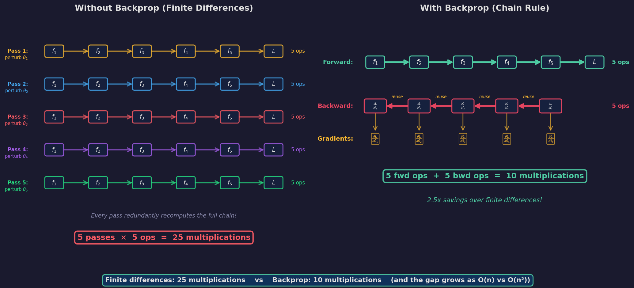
Seeing the Savings: A Chain of 5
Now scale to a chain of 5 functions:
$$x \xrightarrow{f_1} \xrightarrow{f_2} \xrightarrow{f_3} \xrightarrow{f_4} \xrightarrow{f_5} \hat{y} \xrightarrow{\mathcal{L}} \text{loss}$$
Without backprop (finite differences):
- Perturb $\theta_1$: run all 5 layers → 5 operations
- Perturb $\theta_2$: run all 5 layers → 5 operations
- ... repeat for each of 5 parameters
- Total: 25 operations (5 passes × 5 ops)
Every single pass redundantly recomputes the same intermediate values through layers that weren't even perturbed.
With backprop:
- Forward pass: 5 operations
- Backward pass: compute $\frac{\partial \mathcal{L}}{\partial f_5}$, reuse it for $\frac{\partial \mathcal{L}}{\partial f_4}$, reuse that for $\frac{\partial \mathcal{L}}{\partial f_3}$, and so on. Each step is one multiplication, reusing the number you just computed. 5 operations.
- Total: 10 operations (1 forward + 1 backward)
That's a 2.5× savings — and notice the pattern:
| Chain length $n$ | Finite differences | Backprop | Ratio |
|---|---|---|---|
| 2 | 4 | 4 | 1.0× |
| 5 | 25 | 10 | 2.5× |
| 10 | 100 | 20 | 5× |
| 100 | 10,000 | 200 | 50× |
| $n$ | $n^2$ | $2n$ | $n/2$ |
Finite differences scales as $O(n^2)$. Backprop scales as $O(n)$. The savings grow linearly with depth.
The Key Insight: Reuse of Actual Numbers
Here's what makes backprop work, stated as plainly as I can. Consider computing $\frac{\partial \mathcal{L}}{\partial \theta_3}$ in our 5-layer chain:
$$\frac{\partial \mathcal{L}}{\partial \theta_3} = \underbrace{\frac{\partial \mathcal{L}}{\partial f_5} \cdot \frac{\partial f_5}{\partial f_4} \cdot \frac{\partial f_4}{\partial f_3}}_{\text{shared with } \theta_1 \text{ and } \theta_2} \cdot \frac{\partial f_3}{\partial \theta_3}$$
Now look at $\frac{\partial \mathcal{L}}{\partial \theta_2}$:
$$\frac{\partial \mathcal{L}}{\partial \theta_2} = \underbrace{\frac{\partial \mathcal{L}}{\partial f_5} \cdot \frac{\partial f_5}{\partial f_4} \cdot \frac{\partial f_4}{\partial f_3}}_{\text{same prefix!}} \cdot \frac{\partial f_3}{\partial f_2} \cdot \frac{\partial f_2}{\partial \theta_2}$$
The first three factors are identical. In finite differences, you'd recompute them from scratch. In backprop, the quantity $\frac{\partial \mathcal{L}}{\partial f_3}$ is a single number that you already computed and stored. You just multiply it by one more local derivative to get $\frac{\partial \mathcal{L}}{\partial f_2}$, and so on down the chain.
This is the entire trick: backprop computes and caches a running product from the output backwards. At each layer, it extracts the gradient for that layer's parameter (one multiplication) and extends the running product one step deeper (one more multiplication). No chain is ever recomputed — just extended.
In real networks, "one parameter per layer" is unrealistic — layers have weight matrices with many parameters. But the same principle applies: the backward pass computes $\frac{\partial \mathcal{L}}{\partial f_k}$ (the gradient with respect to layer $k$'s output) once, then uses it to compute gradients for all of layer $k$'s parameters simultaneously. The cost of the backward pass is proportional to the cost of the forward pass, regardless of how many parameters the network has.
Complexity Summary
For a network with $P$ total parameters and $n$ layers:
| Method | Cost per gradient | Scales with |
|---|---|---|
| Finite differences | $O(P \cdot n)$ | Parameters × depth |
| Backpropagation | $O(n)$ | Depth only |
This is why deep learning works at scale. It's not a symbolic trick or a mathematical curiosity — it's the algorithm that makes training neural networks computationally tractable. Without it, we'd still be limited to networks small enough to differentiate by hand or by finite differences.
Further Misconceptions
"Gradient Descent Finds the Best Solution"
It doesn't. It finds a local minimum — a point where the gradient is zero and the loss is lower than all nearby points. In a high-dimensional loss landscape, there are astronomically many local minima.
The surprising empirical finding is that in high dimensions, most local minima are about equally good. The truly bad minima are rare. So gradient descent doesn't need to find the global optimum — it just needs to avoid the few pathological basins, and the stochastic noise usually takes care of that.
"Learning Rate Is Just a Speed Knob"
It's also a resolution knob. A large learning rate takes big steps, which means the linear approximation (the gradient) is less accurate for each step. This causes you to overshoot narrow valleys. A small learning rate takes tiny steps within the region where the gradient is trustworthy, but you might get trapped in sharp minima that generalize poorly.
The learning rate affects which solution you find, not just how fast you find it. Bigger steps implicitly bias you toward wider, flatter minima. This is part of why learning rate schedules (starting large, annealing small) work well: explore broadly first, then refine.
"Deeper Networks Are Harder to Train"
This used to be true. In deep networks, gradients computed via backprop pass through many layers of multiplication. If the per-layer derivatives are consistently less than 1, the gradient shrinks exponentially (vanishing gradients). If they're consistently greater than 1, it explodes.
Residual connections, layer normalization, and careful weight initialization largely solved this. The gradient doesn't vanish if you give it a skip connection to travel through. Modern networks with hundreds of layers train stably, which would have seemed impossible twenty years ago.
The Point
Gradient descent is conceptually simple: compute the direction of steepest decrease, take a step. But the simplicity hides important structure. The gradient is local, it lives in parameter space (not on the loss surface), it depends on which data you're evaluating on, and the noisy version works better than the exact version. Understanding these details isn't pedantic — it's prerequisite to understanding where training breaks and where safety assumptions depend on optimization behaving the way you expect it to.
Written by Austin T. O'Quinn. If something here helped you or you think I got something wrong, I'd like to hear about it — oquinn.18@osu.edu.