This post starts with a simple question — how would you tell if two neural networks learned the same thing? — and builds to a case where the standard answer is dangerously wrong.
How would you compare two networks?
Suppose you train two neural networks on the same task from different random initializations, and both get 99% accuracy. Did they learn the same thing?
You can't just compare the raw activation values. To see why, think about a simpler example. Imagine two spreadsheets tracking student performance. One has columns [math_score, reading_score]. The other has columns [total_score, score_difference]. Both contain the same information — you can convert between them with simple arithmetic — but the raw numbers look completely different. A student with (90, 80) in the first spreadsheet would be (170, 10) in the second.
Neural networks have the same problem. Two networks can represent identical information in different coordinate systems. Neuron 47 in network A might encode the same feature as neuron 183 in network B, or the same feature might be spread across dozens of neurons in a different combination. Comparing raw activation numbers is meaningless.
So what you want is a comparison that ignores these superficial coordinate differences and asks: is the underlying structure the same?
Rotation invariance seems like a good idea
Here's where the intuition starts. The relationship between those two spreadsheets is a rotation (plus scaling) — a change of coordinate system that preserves all the geometric relationships between data points. Students who were close together in [math, reading] space are still close together in [total, difference] space. The shape of the data cloud is the same; it's just been rotated.
A natural design choice: make your comparison metric rotation-invariant. If two networks organize their data the same way but in rotated coordinate systems, the metric should see them as identical. The coordinate system is arbitrary — what matters is the structure.
Centered Kernel Alignment (CKA) does exactly this. You feed both networks the same inputs, collect their internal activations, and CKA computes a score between 0 and 1. It's invariant to rotation and isotropic scaling. High CKA means "same structure, possibly in different coordinates." Low CKA means "genuinely different structure."
This sounds right. Two networks that learned the same features in different coordinate systems should count as similar. CKA is the most popular representation similarity metric in the field, used in hundreds of papers. The Platonic Representation Hypothesis uses high CKA as evidence that models converge toward a shared representation of reality.
But rotation invariance has a hidden assumption: it assumes the coordinate system is arbitrary. What if it isn't? What if the specific orientation of the representations — not just their shape — is where the computation lives?
The experiment
I wanted a setup where I could control everything. Same architecture, same data, same hyperparameters — the only thing that changes is the random seed used to initialize the weights.
I trained 40 small transformers on integer addition: the model sees 003+456= and has to produce 0459. Two sizes: a small one (10K parameters, 20 seeds) and a larger one (69K parameters, 20 seeds). Standard training — AdamW optimizer, cosine learning rate schedule, 50 epochs.
The small model sits right at the capacity edge, and that's the key to the experiment. Some random seeds produce models that learn addition perfectly (11/20 reach ≥99% accuracy — I'll call these "good" models). Other seeds produce models that never figure it out (5/20 stay below 20% — "bad" models). Same everything. Different random initialization. Some learn, some don't.
This gives us a natural test: can CKA tell which models actually learned addition?
Three metrics, three contradictory answers
I measured the similarity between these models three different ways. The results are... uncomfortable.
| Metric | What it says | Value |
|---|---|---|
| CKA | "Nearly identical" | 0.97 |
| Probe transfer | "Completely incompatible" | $R^2 = -32$ |
| Weight transplant | "Completely incompatible" | 0% (all 20 configs) |
Let me unpack each of these.
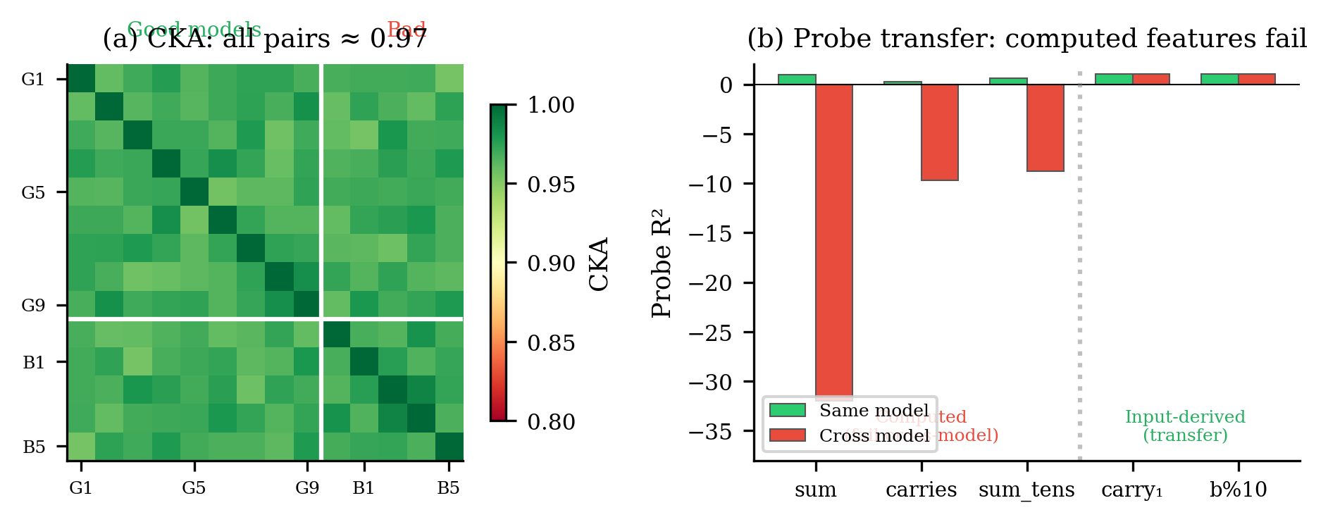
CKA says they're the same. Good-good model pairs score CKA = 0.97. But here's the problem: good-bad pairs — a model that learned addition paired with one that didn't — also score 0.97. CKA literally cannot tell models that solve the task from models that fail.
Probes say they're different. A linear probe is a simple test: train a small linear model on one network's activations to predict the answer, then test it on another network's activations. If the probe transfers, both networks encode the answer the same way.
Within a single model, the probe works beautifully ($R^2 = 0.995$). Cross-model? $R^2 = -32$. That's not just bad — it's worse than predicting the mean every time. The probe's predictions are anti-correlated with reality.
Transplants say they're different. Take two models that both solve addition at 99%+ accuracy. Copy any subset of weights from one into the other — attention heads, MLP layers, embeddings, layer norms, any combination. I tested 20 different configurations across 5 model pairs. Every single partial transplant yields 0% accuracy. Copy everything and you get 100% back. There is no "addition module" you can move between models. The computation is distributed across all weights and co-adapted with everything else.
Why does this happen?
Remember the spreadsheet analogy? Rotation invariance works when the coordinate system is arbitrary — when rotating the data doesn't change what it means. But think about what happens if 90% of your spreadsheet's variance is in one column (say, "total score"), and the interesting stuff (who's good at math vs. reading) lives in the much smaller remaining variation. A rotation-invariant metric would be dominated by "total score" and barely notice the math/reading distinction. Two spreadsheets that agree on total score but completely disagree on math vs. reading would look "almost identical."
That's exactly what's happening here.
To see it, we need one concept: principal components (PCs). When you have high-dimensional data (like network activations), PCA finds the directions of greatest variation. PC1 is the direction capturing the most variance, PC2 captures the most remaining variance, and so on.
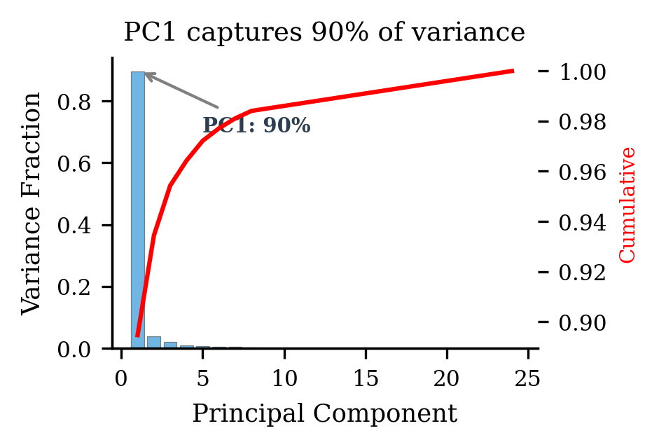
In my models, PC1 captures 90% of the activation variance. That's enormous — 90% of what's "happening" in the activation space is explained by a single direction. And what does that direction encode? The input structure. Roughly, how big $a + b$ is. Every model learns this — good or bad, capable or incapable. It's just reflecting what the input looks like. It's the "total score" column.
The actual computation — carrying digits, propagating sums, producing the right answer — lives in the remaining 10%. The quiet subspace that PC1 drowns out. It's the "math vs. reading" distinction that the rotation-invariant metric can't see.
Now here's CKA's problem. CKA weights components by the square of their variance. When one component holds 90% of the variance, it contributes $(0.9)^2 = 81%$ of CKA's score just by itself. The formula simplifies to roughly:
$$\text{CKA} \approx \cos^2\theta_{11}$$
where $\theta_{11}$ is the angle between the two models' first principal components. Since all models encode the same input structure in PC1, that angle is near zero, so CKA is near 1. Back to the spreadsheet: CKA is comparing total scores and reporting "these students are basically the same," while the math-vs-reading distinction — the part that actually matters — is invisible.
I tested this directly
If the theory is right — CKA is dominated by PC1, and the useful differences live elsewhere — then removing PC1 should change CKA's absolute value but not help it distinguish good from bad models. Here's what happens:
| PCs removed | Good–Good CKA | Good–Bad CKA |
|---|---|---|
| 0 | 0.969 | 0.976 |
| 1 | 0.544 | 0.527 |
| 2 | 0.254 | 0.273 |
| 5 | 0.157 | 0.134 |
| 10 | 0.099 | 0.105 |
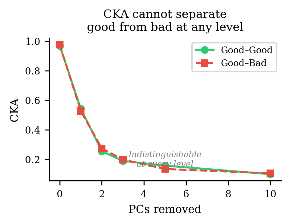
CKA drops (removing PC1 kills most of the signal it was looking at) but the gap between good-good and good-bad stays at zero at every level. The computational differences aren't just hiding behind PC1 — they're hiding behind all the high-variance components. CKA is structurally incapable of detecting them.
It's not just CKA
I hoped other metrics would do better. I tested five activation-based similarity metrics:
| Metric | Good–Good | Good–Bad |
|---|---|---|
| Linear CKA | 0.969 | 0.976 |
| RBF CKA (Gaussian kernel variant) | 0.975 | 0.978 |
| Procrustes distance (rotation-optimal alignment) | 0.113 | 0.103 |
| RSA (comparing internal distance patterns) | 0.870 | 0.886 |
| Cosine similarity (flattened) | −0.004 | 0.003 |
Procrustes distance was specifically designed as a more sensitive replacement for CKA. It also fails. RSA (Representational Similarity Analysis) compares whether models find the same inputs similar to each other — also fails. The problem isn't one particular metric. It's the entire approach of comparing activations when a dominant shared component drowns out the interesting variation.
What actually works: looking at the weights
On the same 40 models where every activation metric is blind, looking directly at the weight matrices detects the difference cleanly.
For modular arithmetic variants (addition mod some prime $P$ — a cleaner version of the same task), the Fourier spectrum of the input projection weights separates capable from incapable models with zero errors ($p = 1.4 \times 10^{-11}$). This works because the discrete Fourier transform diagonalizes modular addition — models that learn the operation develop spectrally sparse weights, and models that don't have diffuse spectra.
On the original 40 integer addition models, a weight-space detector correctly identifies 9/11 successful models and rejects 4/5 failures. CKA provides zero discriminative signal — literally at chance (AUC = 0.50).
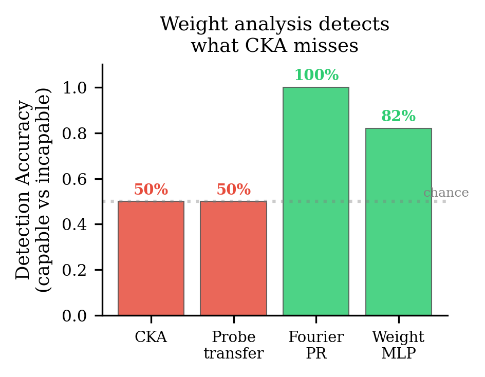
The activations show you what the model sees. The weights show you what the model does.
The sharp boundary in probe transfer
This is the result that made the mechanism click for me. Whether a feature transfers between models depends entirely on whether it requires computation:
| Feature | What it needs | Within-model $R^2$ | Cross-model $R^2$ |
|---|---|---|---|
| sum ($a+b$) | Computation (carry logic) | 0.995 | −32 |
| total carries | Computation | 0.24 | −9.7 |
| sum mod 10 | Computation | 0.60 | −8.8 |
| carry (ones digit) | Just look at the input | 1.00 | 1.00 |
| $b$ mod 10 | Just look at the input | 1.00 | 1.00 |
The boundary is binary. Features you can read off the input — things that live in the shared PC1 subspace — transfer perfectly. Features that require the model to actually compute something — things that live in the model-specific remaining subspace — don't transfer at all. CKA sees only the shared part. The computation is invisible to it.
What transplant failure tells us
The complete failure of weight transplants — every partial configuration, every pair — tells us something important about how these models organize internally.
Fine-tuning after transplant reveals a hierarchy:
| Components transplanted | Direct accuracy | After fine-tuning |
|---|---|---|
| Full transplant (all) | 99.0% | — |
| Embeddings + layer 0 | 0% | 35.5% |
| All except MLP | 0% | 30.0% |
| Output head only | 0% | 12.0% |
| All except embeddings | 0% | 0.8% |
The embeddings anchor everything. If you transplant the embeddings (the model's "dictionary" for converting tokens to vectors), the other weights can partially adapt — 35.5% accuracy after a few epochs of fine-tuning. But transplant everything except the embeddings? The model recovers almost nothing (0.8%). The input representation defines the coordinate system for the entire computation. Change the coordinates and nothing else fits.
This matters for mechanistic interpretability. If you find a circuit in one model — "these attention heads implement carry propagation" — that circuit exists in that model's coordinate system. A model trained from a different seed may implement the same operation using completely different weight configurations. The algorithm is the same. The implementation is model-specific.
So what should you actually use?
The PC-removal diagnostic (three lines of code)
For any study using CKA to compare representations:
- Compute PCA on each model's activations.
- Remove the top $k$ principal components ($k = 1, 3, 5$).
- Re-compute CKA on the residual activations.
- If CKA drops sharply but the difference between your experimental groups doesn't change, CKA is dominated by shared structure rather than computation.
A quick reference:
| Use case | Recommendation |
|---|---|
| Geometric similarity (manifold shape) | CKA is valid |
| Functional equivalence (do they compute the same thing?) | Use probe transfer. CKA is unreliable |
| Comparing checkpoints | Run the PC-removal test first |
| Safety audit / capability detection | Weight-space analysis detects what activation metrics miss |
| Any CKA use | Report the PC1 variance fraction. If it's above 80%, be suspicious |
Why this matters for safety
This isn't just a methodology paper. If we're using representation similarity to argue that models "learn the same thing" — and building safety claims on that convergence — we need the metric to actually detect functional differences.
CKA doesn't. A model that appears representationally identical to a safe, well-understood model may be computing something entirely different in the subspace CKA can't see. Weight inspection may complement behavioral testing for capability evaluation — particularly when behavioral testing is expensive, incomplete, or when models may conceal capabilities under standard probing.
Limitations I want to be honest about
This is demonstrated on small transformers (10K–69K parameters) on integer addition. Whether PC1 dominance and CKA failure occur at scale — large language models, vision transformers, models with learned embeddings and many tasks — is genuinely an open question. The variance structure might look very different.
The weight-space detectors work on modular arithmetic with clean structure. Whether you can detect capabilities from weights in frontier models remains unknown. This is a proof of concept, not a production tool.
Paper: Geometric Similarity Is Blind to Computational Structure (AAAI format, 7 pages)
Code: 40 trained transformer models, 25+ analysis scripts. Reproducible from a single seed list.
Written by Austin T. O'Quinn. If something here helped you or you think I got something wrong, I'd like to hear about it — oquinn.18@osu.edu.